Material Hardness : Effect of Carbon Content & Heat Treatment on Material Hardness

Understand the material hardness and the effect of carbon content and heat treatment on hardness

This lab work aims to understand the material hardness of different materials and effect of carbon content present in the material on material hardness and the effect of heat treatment of material on material hardness.

To achieve the aim of this lab work the following mentioned objectives have to be completed in said sequence

1. Develop a comprehensive understanding of methods used for measuring material hardness

2. Develop a comprehensive understanding of the effect of carbon percentage on material hardness

3. Develop a comprehensive understanding of the effect of heat treatment on material hardness

4. Perform a hardness test to measure material hardness

5. Perform hardness test after increasing carbon content

6. Perform hardness test after heat treatment of material

7. Develop a comprehensive conclusion about the work

Material Hardness

Material hardness can be defined as the material's ability to resist indentation. In more de, tail it can be defined as the material's ability to resist localized plastic deformation which is in the shape of indention and scratch. 

Material hardness is also a great way to understand material wear resistance as it is observed that the greater the material hardness greater the material wear resistance.

Another important relation of hardness with the material is that the material hardness is roughly proportional to material strength. 

Material Hardness Testing

Material hardness tests are very simple, easy, and straightforward to perform as the only thing needed to be done in a material hardness test is to produce a dent in the material and then the force or load needed to produce a dent in the material is used to measure the material and hardness. 

Hardness measured during the experiment is usually a dimension less number only that defines the level of hardness of material means hardness is a unit less quantity. 

Hardness tests are destructive tests by the nature of the f testing material but in some cases, these tests can be considered non-destructive tests as they only create a small dentmaterials'ssl's surface and the material can be used in any way possible after the test. 

There are three different hardness testing methods namely as 

• Brinell hardness test 
• Rockwell hardness test
• Vicker hardness test

differenceconsciencee in the type of hardness test is based on the type of indenter used in the experiments, the load applied during the experiments, and how the load is applied during the experiment. 

There are three different types of indenters used for the hardness test. F first is the ball indenter made from steel and has a diameter of 10 mm in most cases. Second is the diamond cone and third is a diamond pyramid.

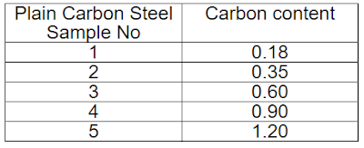
To check the effect of carbon content and heat treatment on the material, different samples of material are provided as per below mention details

For checking carbon content

Material Content

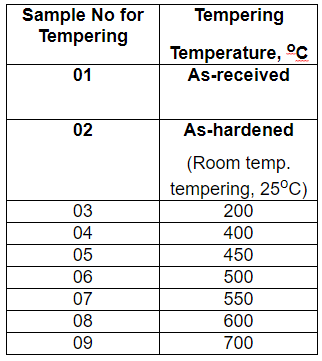
For heat treatment

• As-received sample
• The sample hardened at 1300 C and quenched
• Samples were quenched and tempered for 1 hour at various temperatures from 200 C to 750 C.

Temperature Effect on Material

Procedure for Material Hardness Testing

Following are the steps needed to perform a hardness test on the material

• The first step is the setting up of the apparatus for the experiment and this includes ensuring that the apparatus is placed on a horizontal surface, no initial load is applied on the machine, and related indenter is installed properly 

• The second step is preparing the sample for the test and that includes making a clean horizontal surface with dimensions as per the standard provided.

• The third step is to place the sample material on the anvil of the machine in a manner that it is directly below the indenter

• The fourth step is to move the elevation screw of the machine to move the anvil up so that the indenter and workpiece almost touch each other

• The fifth step is to select the load as per the type of indenter and then apply the load for a few second

• In the case of Brinell hardness and Vicker hardness manual readings of the dent diameter and diagonal end will be taken respectively and they will be used to calculate the respective hardness number. In Rockwell's case, the hardness number will be available directly on the screen of the machine

• Repeat the process for different samples of the material provided for the test and record the data of each material in the table provided

Results of Material Hardness Test

Table 1 Carbon content and Material Hardness

Rockwell hardness test was performed using the basic method and procedure mentioned above in the procedure section and results were recorded in the Rockwell section of the provided table.

 

Two different values were taken and an average of these values was calculated and then that averaged value was used the hardness value of the material. 

Graph one shows the comparison of carbon content in the material with the material hardness with carbon content on the x-axis and hardness on the y-axis. 

The graph shows that with an increase in carbon content in a material the hardness of the material increase but this increase is up to a certain limit and after that material, hardness start to decrease. 

This is because steels that have more than 0.8 percent Carbon, have a combination of cementite and pearlite in it. 

When more carbon is added to steel, cementite is formed, so it decreases the thickness of the material. 

After a certain limit addition of carbon starts to make the material brittle enough to decrease its hardness.

 

Figure 2 Vicker hardness and carbon content

The Vickers hardness test was performed using the basic method and procedure mentioned above in the procedure section and results were is recorded in the Vicker section of the provided table. 

X and Y values were taken and an average of these values was calculated and then that averaged value was used to calculate the hardness of the material. 

Graph two shows the comparison of carbon content in the material with the material hardness with carbon content on the x-axis and Vicker hardness on the y-axis. 

The graph shows that with an increase in carbon content in the material, the Vicker hardness of the material increase but this increase is up to a certain limit, and after that material's Vicker hardness start to decrease. 

This is because steels that have more than 0.8 percent Carbon, have a combination of cementite and pearlite in it. 

When more carbon is added to steel, cementite is formed and is brittle but hard, so it increases the hardness of the hardnessrial. 

After a certain limit addition of carbon starts to make the material brittle enough to decrease its hardness.

 

Figure 3 Rockwell hardness and tempering temperature

To check the effect of tempering temperature on material Rockwell hardness, Different material samples were prepared at different tempering temperatures. 

The value of each sample was recorded and noted again in the respective temperature column present in the table provided.

Graph three was generated for the effect of temperature on Rockwell hardness with temperature on the x-axis and Rockwell hardness on the y-axis. 

Graphs show that an increase in tempering temperature has a very small effect on hardness initially where hardness increases very little. 

This small increase in hardness is up to 550-degree temperature and after that for 600 and 700-degrtemperaturesure hardnestartsart to decrease steadily but continuously.

An increase in material hardness is because temperature removes the internal stress and allows the material to have stronger bonds between atoms but this is up to a certain limit after that increase in temperature makes the material soft which reduces hardness.

 

Figure 4 Vicker hardness and tempering temperature

Different material samples were prepared at different tempering temperatures, to check the effect of tempering temperature on material Vicker hardness. 

The hardness Value of each sample was recorded and noted again in the respective temperature column present in the table provided. 

Graph four was generated for the effect of temperature on Vicker hard with temperatureurer h o the x-a s and Vicker hardness on the y-axis. 

The Graphsshowsw that an increase in tempering temperature has a very sharp effect on hardness lately where hardness increases very sharply. This sharp increase in hardness is at 500 and550 degrees temperature and after that 600 and 700 degrees temperature hardness start to decrease steadily and continuously. 

An increase in material hardness is because temperature removes the internal stress and allows the material to have stronger bonds between atoms but this is up to a certain limit after that increase in temperature makes the material soft which reduces hardness.

Conclusion on Material Hardness Test 

This lab work aims to understand the material hardness of different materials and effect of carbon content present in the material on material hardness and the effect of heat treatment of material on material hardness. 

To check the effect of carbon content and heat treatment on the material, different samples of material were provided with the following carbon contents (in weight %): 0.18, 0.35, 0.60, 0.90, 120, and samples hardened and quenched at 1300 C and set of samples tempered and quenched for one hr at temperatures ranging from 200 C to 700 C. 

The graph shows that with an increase in carbon content in the material the hardness of the material increase but this increase is up to a certain limit and after that material, hardness start to decrease. 

This is because steels that have more than 0.8 percent Carbon, have a combination of cementite and pearlite in it. When more carbon is added to steels, cementite is formed and is brittle but hard, so it increases the hardness of the material. 

The Graphs show that an increase in tempering temperature has a very sharp effect on hardness lately where hardness has increased very sharply. 

This sharp increase in hardness is at 500 and 550-degree temperature and after that for 600 and 700-degree temperature hardness start to decrease steadily and continuously. 

An increase in material hardness is because temperature removes the internal stress and allows the material to have a stronger bond between atoms but this is up to a certain limit after that increase in temperature makes the material soft which reduces hardness.

Working of an Air Condition unit

Air conditioning unit, or air-con, AC, A/C, is the process where heat and/or moisture is removed from a building or interior space to improve the comfort of the occupants. 

It applies to both residential and commercial spaces. It is used to improve the comfort of both humans and animals. 

Sometimes, these systems are also used to dehumidify and cool spaces occupied by heat-producing devices such as computer servers as well in storage rooms with delicates stored items such as artworks. 

Air-conditioning systems are equipped with a fan(s) that are used in the distribution of conditioned air to areas of interest to improve the comfort of the occupants. 

The cooling and/or heating is achieved through the refrigeration cycle. 

However, sometimes free cooling or evaporation is also used. In some ACs, desiccants are used to remove and/or add moisture from the air.

The current experiment involves an analysis of an air-conditioning system by use of a psychrometric chart as well as a practical measurement of various components. The two sets of results are then compared and conclusions made. 

Also covered is the research and review on air-conditioning plants as far as environmental issues, energy issues, health issues, and policies are concerned.

Parts of Air conditioning Unit

A standard air conditioning unit consists of four different and basic components that work together to provide air which is conditioned at the required temperature and humidity. Basic components of an air conditioning unit are

1. Compressor

2. Condenser

3. Expansion valve

4. Evaporator

Working of Air Condition Unit

The process of the air conditioning unit starts from the compressor stage where refrigerant is compressed to the required pressure. 

Compressor on the air condition unit work as a container for the refrigerant and also as the main power consuming and producing unit of the AC system. 

Compressing the refrigerant increases its pressure and temperature where pressure is required to move the refrigerant throughout the air conditioning system. 

The increase in temperature of the refrigerant is unwanted and it is reduced in the condenser stage of the air conditioning system. 

Condenser condenses the refrigerant into the liquid form and reduces its temperature by reducing the temperature of the refrigerant. 

Condenser is a heat exchanger which removes heat from the hot fluid by passing it to the much lower temperature outside air. 

After condenser the refrigerant is passed to the expansion valve which is designed to reduce the pressure of the refrigerant. Expansion valve reduce the pressure of the refrigerant by allowing it to expand suddenly. 

This reduces the temperature and pressure of the refrigerant and thus enables the refrigerant to work as a low temperature fluid. 

In last stage of the air conditioning system the refrigerant enters the evaporator which is also a heat exchanger and it is the only indoor unit of the air conditioning system. 

Evaporator works to reduce the temperature of the indoor air by exchanging the indoor air heat with the much lower temperature refrigerant. 

Objectives

The overall objective of the experiment was to familiarize oneself with energy technology concepts and principles while solving a practical problem. 

This was to be accomplished through practical measurement of data, analyze the data, and appraise the results while presenting the outcome of the experiment in a report format.

Procedure of an Air Condition unit

The procedure for the current experiment was to fill all the relevant sections in the datasheet provided. This was accomplished by reading all the relevant values from the measuring instruments three times and while entering the data in the datasheet. For calculations, the average values were utilized.

Results and Calculations Air Condition unit

The table below shows the data collected during the experiment.

Air condition unit experimental data

Dry air flow rate

The air that flow into the air conditioning system for conditioning is added into the point D of the system. The mass flow rate of the dry air that moves into the system can be calculated from following formula. 

m ̇_a=0.05717* √(Z/v_D )

In the above formula v_Dis the specific volume of the air based on its dry bulb temperature and wet bulb temperature and z is the pressure differential in the water column due to the flow of air over it and it is measured in mmH2O. 

To measure the specific volume to calculated the mass flow of the dry air moving into the air conditioning system the dry bulb temperature and wet bulb temperature of air moving into the system are marked on psychometric chart the point at which their respective line cut each other gives the value of specific volume. 

m ̇_a  = 0.0517 * √(4.6/0.895)

m ̇_a  = 0.1172  kg_(dry_air)/S

Part-2: Water added to the system

The water that flow into the air conditioning system for conditioning the air as required is added into the system between point A and B of the system. 

The mass flow rate of the wet air that moves into the system can be calculated from following formula. 

m ̇_(water_AB )  = m ̇_a  * (ω_B  -〖 ω〗_A )

In the above formula ω_Bis the water content in air at point B, based on the air dry bulb temperature and wet bulb temperature of air at the point B. 

Similarly ω_Ais the water content in air at point A, based on the air dry bulb temperature and wet bulb temperature of air at the point B. m ̇_a is the mass flow rate of the dry air moving in the system from point A to the point B. 

To measure the water content in the air added at the point B, the dry bulb temperature and wet bulb temperature of air at the point B in the system are marked on psychometric chart, the point at which their respective line cut each other gives the value of water content in the air at point B. 

similarly when the dry bulb temperature and wet bulb temperature of air at the point A in the system are marked on psychometric chart, the point at which their respective line cut each other gives the value of water content in the air at point A.

m ̇_(water_AB )  = 0.1172 * (0.020 - 0.0098)

m ̇_(water_AB)  = 0.0012  kg/s

Part-3: Energy balance between sections A and B

Heat and Work transfer rate

Two different boilers one with power of 1 KW and one with power of 2 KW generate heat for this system. 

Similarly two identical preheaters are also provided each with power of 1 KW.

(V^2/R)_(Pre_heater)+ (V^2/R)_(Boiler_2kW)+ (V^2/R)_(Boiler_1kW)+ Fan power_(@235.7V)=  〖235〗^2/47.4  +  〖235〗^2/23.9  +  〖235〗^2/58.7  + ≈ 135 = 4551.55  W ≈ 4.55  kW

Enthalpy change rate

Due to the conditioning of the air in the air conditioning system the enthalpy of the system changes at every step and rate at which it changes is called the enthalpy rate. 

It depends on the mass flow of dry air between the point A and B and the enthalpy of the air at the point A and B and the mass flow of water added into the system between the point A and B. 

The enthalpy of air depends on the dry bulb temperature of air, so enthalpy of air at point A depends on the dry bulb temperature of point A and enthalpy of air at point B depends on the dry bulb temperature of point B. 

Putting the value of dry bulb temperature in steam table will give the value of enthalpy of the respective point.

Enthalpy change rate= m ̇_a  * (h_B  -〖 h〗_A )  - m ̇_(water_AB )  *〖 h〗_f

At DBT_A (18.93) C,

h_f  ≈ 54  kJ/kg

Therefore;

Enthalpy change rate = 0.1172 * (85.5 - 43)  - 0.0012 * (54)  ≈ 4.92  kW

Part-4: Rate of water removed

by use of the psychrometric chart

The water that flow out of the air conditioning system for conditioning the air (as required) is removed from the system between point B and C of the system. The mass flow rate of the water content out of the system can be calculated from following formula. 

m ̇_(water_BC )  = m ̇_a  * (〖 ω〗_B  - ω_C  )

In the above formula ω_Bis the water content in air at point B, based on the air dry bulb temperature and wet bulb temperature of air at the point B. 

Similarly ω_cis the water content in air at point C, based on the air dry bulb temperature and wet bulb temperature of air at the point B. m ̇_a is the mass flow rate of the dry air moving in the system from point B to the point C. 

To measure the water content in the air removed at the point C, the dry bulb temperature and wet bulb temperature of air at the point C in the system are marked on psychometric chart, the point at which their respective line cut each other gives the value of water content in the air at point C. 

similarly when the dry bulb temperature and wet bulb temperature of air at the point B in the system are marked on psychometric chart, the point at which their respective line cut each other gives the value of water content in the air at point B.

m ̇_(water_BC )  = 0.1172 * (0.020 - 0.0145)

m ̇_(water_BC )  = 0.00064  kg/s

by measurement of the condensate collected

The amount of water removed from the system can also be measured directly from the water collected in the condenser section air conditioning system. 

The mass flow of water moving out of the system depends on the water quantity collected in the condenser.

m ̇_(water_BC )  =  (164 * 〖10〗^(-6)  * 1000)/300  

m ̇_(water_BC)  = 0.00055  kg/s

Part-5: Heat input to the air using SFEE between sections C and D

Due to the conditioning of the air in the air conditioning system the heat moves into the system and rate at which it moves is called the heat addition rate. 

It depends on the mass flow of dry air between the point C and D and the enthalpy of the air at the point C and D. 

The enthalpy of air depends on the dry bulb temperature of air, so enthalpy of air at point C depends on the dry bulb temperature of point C and enthalpy of air at point D depends on the dry bulb temperature of point D.

Putting the value of dry bulb temperature in steam table will give the value of enthalpy of the respective point.

By use of the psychrometric chart

Heat Input,Q ̇  = m ̇_a  ( h_D  - h_C  )

Heat Input,Q ̇  = 0.1172 ( 71.5 - 58 )

Heat Input,Q ̇   = 1.58  kW

By heat addition

Heat Input,Q ̇=+(V^2/R)_(Boiler_2kW)=〖235〗^2/23.9≈2.31 kW

Discussion on Working of an Air Condition Unit

Part-1: Accuracy of results stating possible errors

There was a discrepancy between the computed values and the expected changes of enthalpy in the refrigeration system.

The heat added to the system was approximately 4.55 kW while the empathy change indicated that the heat received was 4.92 kW. 

Taking the heat determined from the supplied power as the base value, the discrepancy is 8.13%. 

The rate of water removed was determined to 0.00064 kg/s from the psychrometric chart while the condensate was 0.00055 kg/s from the experiment. 

This resulted in a discrepancy of 18%. Finally, the heat added to air was determined to be 1.58 kW from the psychrometric chart while the actual heat added was 2.31 kW resulting in a discrepancy of 31.6% discrepancy.

These discrepancies can be attributed to several issues as summarized below;

Approximation of various values from the psychrometric chart especially where decimal values are encountered. 

This can also emanate from the complexity of the psychrometric chart where various values have to be read/determined from the same system point.

Human errors when reading the various values from the psychrometric chart and thus errors in calculation.

Faulty measuring instruments such as manometer, timer, and thermometers during the experiment.

The experiment can be improved through;

Mastery of using the psychrometric chart in solving the refrigeration and other thermodynamic systems.

Calibration of the measuring instruments to be used in the data collection during the experiment.

Issues Related to air conditioning units

Environmental issues

Air-conditioning plants consume a lot of energy. This means air or/and water and/or sound pollution at the source of the electricity. A rage number of these plants uses chemicals such as CFCs, HCFCs, and HFCs as the colling agents.

When such agents are released to the environment either accidentally or at the end of life, they have negative effects on the ozone layer and thus leads to global warming over time.

The recent times, many air-conditioners are being manufactured from plastics. If disposed to the environment, plastics can be detrimental as they are non-biodegradable. However, a large percentage of plastics can be recycled.

Energy Issues

Air-conditioning plants consume a lot of energy for them to function as expected. This deprives other energy needs as well as being very expensive to operate especially during extreme weather conditions (cold or hot) (Davis and Gertler, 2015).

Health Issues

A large percentage of the air-conditioning plants use ducts in their operations. Over time, these ducts accumulate dust and bacterial such as Legionella bacteria which causes Legionnaires' disease (Orkis et al., 2018). 

Whenever the air-conditioning plant is turned on, the dust and other contaminants are released to the surroundings and are inhaled by the users and thus affecting the health of people. 

 While there are ductless air-conditioners in the market, they are expensive to acquire. On the other hand, air-conditioning can save lives, especially in extreme weather conditions. 

Air conditions can help people with asthma as they are designed to condition are and also to filter it before provided it to the users. Filter removes dust and also harm full gases and this help people with breathing problems Orkis et al., 2018).

Policies

Montreal Protocol – This is an international treaty that was designed for ozone layer protection. it was signed on 26th August 1987. 

The treaty aims to phase out the production of various products that depletes the ozone layer such as those used in air-conditioning plants. The treaty has 46 signatories and ratified by 20 states.

The new model guidelines for room air conditioners and refrigerators – The guidelines require energy-efficient appliances as well as the use of refrigerants with a lower global warming potential.

United for Efficiency (U4E) guidelines - This guide focuses on room air conditioners. 

 It is intended to provide policymakers with information and best-practice case studies on how to promote energy-efficient and climate-friendly room air conditioners in their respective national markets.

Lab Report: To Study the Buckling of Struts

Over View of Buckling of Struts

Buckling of strut is an important phenomenon in engineering. In this experiment buckling of struts for different materials has been studied. Materials used in this study were aluminum, steel and brass. 

Ten samples of circular struts of similar diameter but of different length were taken for each material type. 

Tensile testing machine was used to perform the experiment. Two different methods were used to find the buckling load and stress theoretically. 

Euler formula which is usually used for long struts was used to calculate the amount of buckling load and stress in the samples.

Rankine’s formula was also used to calculate the load and stress in all the samples of different materials. 

The data for experimental, Euler’s formula and Rankine’s formula was then gathered, manipulated and put in tabular form to make it eye-catching and easily understandable. 

Graph for all materials show that value of stress is very close to experimental values at high slenderness ratio while the difference in the value of stress is quite large at low slenderness values.

Aim

“To Study the Buckling of Struts”

The aim of this experiment is to study different techniques to measure buckling of struts made up of different engineering materials. 

Two methods from theory are also used to calculate the amount of buckling load and stress. The materials included in this study are brass, steel and aluminum. 

Objectives

In order to complete the experiment of buckling of struts, the following pieces of work will be completed in the given order.

• Gathering data from the apparatus to complete the test log sheet
• Calculation of buckling load using Euler’s theory
• Calculation of buckling load using Rankine’s theory
• Comparison of experimental and theoretical value for each material
• Discussion on the results 

Theory on Buckling of Struts

Basics of buckling and struts

Struts are an important engineering component found in different engineering applications usually installed to bear compressive loads. They can also be used to take tension loads. 

In theory, there are two theories for studying buckling in the struts. One of which is Euler’’s theory and the second is Rankine’ formula.

Formulas and important parameters used in both theories are discussed one by one.

Euler Formula for Buckling

Euler Buckling Theory is a classical theory to find the critical buckling load for the column of any cross-section. 

It is usually adopted to calculate the buckling load in long columns. 

The derivation of Euler’s formula for buckling starts from noting that bending moment in a loaded column and buckled column is ‘Py’. 

Where ‘P’ is the load applied and ‘y’ is the deflection of strut or column. 

This expression is then put into beam deflection equation and appropriate boundary conditions are then applied which leads to the final formula of Euler’s theory of buckling.

Euler’s formula for calculating the buckling load is given as

P_E=(π^2 EI_min)/(L_e^2 )

Where 

‘P_E’ is Euler’s load (Buckling or Crippling) or sometimes known as critical load. It is called critical because increasing load beyond this value will cause the strut or column to buckle. ‘E’ is the Young’s Modulus of column’s material. 

This value will change for all materials. ‘I_min’ is the minimum moment of inertia for a column’s cross section. 

Suppose if the column is rectangular, the moment of inertia for the smaller side will be put into the formula. Because column bends in the direction of smaller dimension. 

But in our study, we are using a circular column, so there will be only one moment of inertia. L_e is the effective length of the column that actually takes part in bending. 

Sometimes, it may happen that complete length of the column does cause bending. 

Euler’s stress can then be calculated by simply dividing P_E by the cross-sectional area of the strut or column.

Rankine’s Formula for Buckling

Rankine’s theory for finding buckling load on strut is used to calculate buckling load in the columns of short, average and large length. 

The column is decided to be short, medium or long based on the l/k ratio. The derivation of Rankine’s formula starts from the statement 

1/P_R =1/P_E +1/P_c 

Where P_R is Rankine’s crippling or buckling load, P_E is Euler Buckling load and P_c is crushing or compressive load. 

For the small sized struts or columns, 1/P_E  becomes almost equal to zero so the Rankine’s buckling load will be equal to P_c. 

Similarly, for the long struts or columns 1/P_c  becomes almost equal to zero and the Rankine’s buckling load will be equal to P_E.

 The mathematical manipulation of above equation leads to the following form of Rankine formula,

P_R=(σ_c A_c)/(1+a〖(Le/k_min )〗^2 )

Where σ_c compressive load, a is the Rankine’s constant whose value will change depending upon the material of the column.

Procedure of Buckling of Struts

• The experiment to find the buckling load is performed on tensile testing machine. Following set of steps are to be performed to complete the experiment.

• First of all, length of column is measured using micrometer or simple steel ruler and value is recorded in mm.

• Cross-sectional area of the each specimen is then calculated from the radius of specimen.

• After that, specimen is placed between the jaws of the machine as per the instructions provided and the buckling test is performed.

• The value of load is printed for each person in the group.

• The value of load is recorded in N (Newton).

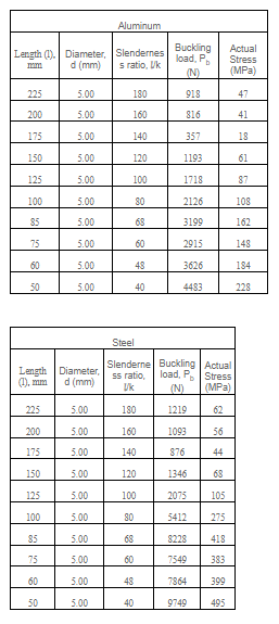
Experimental Results

Discussion on Buckling of Struts

Actual stress, stress using Euler’s formula and Rankine’s formula for Aluminum, steel and brass respectively has been found in this experiment. Figure-1 shows the graph between slenderness ratio and buckling stress for aluminum. 

The results of rankine’s theory are closer to the experimental values at higher slenderness values but initially the error is quite high as initial stress value for Rankine Formula is very low as compared to that of the experimental value. 

While results of Euler’s theory are closer to experimental values at high slenderness ratio but the error is quite high at low values of slenderness ratio.

The result provided by the Euler’s theory area non uniform as the graph show sudden increase and decrease in the stress value for increasing value of slenderness ratio. 

This sudden increase and decrease can only be explained in way that either stress production depends highly on material properties like strength, hardness and ductility or the experimental setup has limitations for this method. 

It also shows that with increasing value of slenderness ratio the stress produce in the truss start to decrease. 

The graph pattern of stress and slenderness ratio is non-linear which show that it depends a lot on other material properties rather than just on the specimen dimensions or slenderness ratio. 

 

In the figure-2 for steel, the pattern is quite similar as in the figure-1 

Where the results of rankine’s theory are closer to the experimental values at higher slenderness values but initially the error is quite high as initial stress value for Rankine Formula is very low as compared to that of the experimental value.

 

Similar pattern in the figure-3 can also be observed for the third type of material which is brass. 

It can be further concluded that Euler’s theory demands extra strength for material which can boost the costs. 

While Rankine’s theory underestimates the material’s strength which can cause serious problem in real life structures.

 

Figure 3- Stress in Brass

Sources of Errors

• Any slippage in grip can distort the measurement.
• Axial misalignment of machine jaws can cause error.
• The large error at low values of slenderness can be due to fact that the grip weight might be ignored

Conclusion on Buckling of Struts

The aim of this experiment was to study different techniques to measure buckling of struts made up of different engineering materials. 

Two methods from theory were used to calculate the amount of buckling load and stress. The materials included in this study were brass, steel and aluminum. 

The results of rankine’s theory are closer to the experimental values at higher slenderness values but Euler’s theory are closer to experimental values at high slenderness ratio but the error is quite high at low values of slenderness ratio. 

It was concluded that Euler’s theory demands extra strength for material which can boost the costs while Rankine’s theory underestimates the material’s strength which can cause serious problem in real life structures.

Diesel Engine Vs Petrol Engine

For Diesel Engine vs Petrol Engine discussion we have written diesel engines advantages over petrol engines. So Following are is a brief comparison of petrol engine and diesel engine

Diesel Engine Vs Petrol Engine 

A diesel engine burns fuel at a high compression ratio instead of using spark plugs and they are also un-throttled which is why diesel engines are more efficient compared to petrol engines.

Comparing Diesel Engine Vs Petrol Engine over thermal efficiency. The thermal efficiency of diesel engines is higher than that of petrol engines which means that they can convert more of the heat supplied into useful mechanical work and waste less of it in the environment.

Diesel engines are low-carbon and other greenhouse gas emitters. Greenhouse gases are responsible for elevating the earth’s temperature. 

Diesel engines work at lower RPMs contrasted with a petrol engine which causes less frictional losses. The pieces of the diesel engine are thicker because of the high pressing factor they need to withstand. 

This makes them more strong along these lines and less inclined to fall flat. Diesel being a light oil likewise greases up the burning chamber each time it's utilized. This additionally makes it last more as less grinding means less wear which thus implies less maintenance is required. 

These engines are worked for more force while being more effective than a petrol engine. The explanation is the pressure proportion. 

As diesel engines are self-touching off, they need to produce sufficient pressing factors in the burning chamber which would make the diesel light. 

This increment in pressure proportion implies more force/torque delivered when ignition happens. The diesel engine likewise has quicker ignition which implies more force/torque too. 

As they produce more force/torque, diesel vehicles are more qualified for pulling substantial things. 

Force decides the rotational power of the vehicle and the more force/torque a vehicle has the more burden it can convey without losing execution. This makes the diesel-controlled vehicle ideal for weighty takes. 

From fewer visits to the service station to more grounded engine parts that don't flop as regularly, diesel engines are more solid than petrol over the long haul. 

They are costlier to fix than petrol however they flop less regularly when contrasted with petrol along these lines making the chances for diesel.

Emissions from Diesel Engines and Effect on Environment and Human Health

Transport has played an important role in escalating climate change and increasing environmental pollution. 

According to a report by the International Energy Agency in 2012, transport contributes to 22% of carbon emissions which is the second largest in the world. 

Transport is the main source of urban pollution especially in the developing world due to the very limited use of carbon control technology. 

Diesel is chemically made up of carbon and hydrogen in different proportions. 

In a diesel engine, fuel is sprayed onto highly compressed air inside the cylinder which ignites the combustion. High pressure inside the cylinder triggers the auto combustion of diesel. 

If we see from an ideal thermodynamic equilibrium perspective, the combustion process should produce CO2 and H2O. But, due to many reasons such as combustion temperature and timing, air–fuel ratio and turbulence, etc., different harmful products are produced during combustion. 

Carbon monoxide (CO) is emitted due to incomplete combustion when the oxidation process does not occur completely. It is largely dependent on the air-fuel mixture. When the air-fuel mixture is rich and the air is deficient, all the carbon can’t burn which causes CO emission. It is a colorless and odorless gas. 

When we inhale air, it is transported to the lungs and subsequently transmitted to the bloodstream. It binds with hemoglobin and hinders its capacity to transfer oxygen. Depending upon the concentration of CO inhaled, it can damage different organs and can also cause confusion and slow reflexes. 

Brief Introduction of Emission Reduction Techniques for Diesel Engines

Due to adverse effects on both humans and the environment, scientists have adopted different methods to reduce emissions. Most of the researchers have worked on to reduced NOx emissions and it has the highest percentage among other pollutants. 

Lean NOx trap (LNT), Exhaust gas recirculation (EGR), and Selective Catalytic Reduction (SCR) are the most focused technologies by researchers. In EGR, exhaust gas is recirculated in the combustion chamber with fresh air. 

LNT technology works by storing NOx under lean mixture conditions and using it when the mixture is rich. SCR is an advanced technology that uses a liquid agent in the exhaust stream of a diesel engine. The 

Separate systems for emission control i.e. Diesel oxidation catalyst (DOC), Diesel particulate filter (DPF), and Selective catalytic reduction (SCR), are also extensively used.

That all for Diesel Engine Vs Petrol Engine Have a great day

Coefficient of Thermal Conductivity

Conduction can be defined as the transfer of electrons from one place to another under a potential difference or heat gradient. It is one of three modes of heat transfer between two or more bodies at different temperatures. 

The other two modes of heat transfer are convection and radiation. Generally, in solids conduction is due to the vibrations of molecules and motion of free electrons. Metals have high number of free electrons which explains that why they are good conductors. 

Thermal conductivity is the extent by which a substance can conduct heat or electricity. Solid, specifically speaking metals, have high thermal conductivity whereas gases have low value of thermal conductivity. The formula for Fourier Law of heat conduction can be given as

Q=kA dT/dx

Where,

Q = Heat flow rate, [Watt]

k = Thermal conductivity of the material, watt/km 

A = Cross-sectional area of the conduction, [m2]

dT = Temperature Difference, [K]

dx = Thickness or length of the material specimen, [m]

Factors Effecting Thermal Conductivity

Thermal conductivity depends upon several parameters.

Material: It highly depends upon the material. As discussed above metals have high thermal conductivity compared to gases. Some non-metal materials can also have higher thermal conductivity compared to metals.

Length: The length of the specimen or material through which heat will flow also affects the thermal conductivity. For a material or specimen whose length is short, the heat will flow easily and faster. But in some cases, thermal conductivity may increase with the increase in length. 

Temperature Difference: Thermal conductivity of a material also varies with change in temperature. In some of the cases thermal conductivity increases with increase in temperature while in some cases it decreases with increase in temperature.

Cross-Section Types: Thermal conductivity is also dependent on the shape of material. Materials. The cross-section type like hollow-shaped or C-shaped can affect the thermal conductivity as well. 

Measurement of Thermal Conductivity

There are two types of techniques which are used to measure the thermal conductivity of a material. The first one is steady-state technique and the second one is non-steady or transient technique.

In the steady state technique for measuring thermal conductivity, measurement is taken when the material whose thermal conductivity is measured is in the thermal equilibrium state. 

The problem with this method is that it takes a lot of time to achieve the equilibrium. Moreover, this method also includes expensive equipment to take the readings correctly.

In the transient or non-steady method, readings are taken during the heating process. It records the readings of thermal conductivity using transient sensors. 

With this method, thermal conductivity can be found relatively quickly.

Increase and Decrease in Thermal Conductivity

For metals thermal conductivity is mainly the function of free moving electrons. With the increase in temperature, the vibrations of electron increases which decreases the passage for moving electrons. 

Hence, it decreases thermal conductivity. For the liquids, thermal conductivity also decreases with increase in temperature.

In the case of gases, increase in temperature will increase the amount of collisions amongst molecules. Thus it increases thermal conductivity. 

Material with Highest Thermal Conductivity

Diamond is considered to have highest thermal conductivity. Solids that have crystalline structures have high thermal conductivity as compared to the solids that have amorphous structures. 

Due to the same reason, thermal conductivity of gases is lower because atoms are arranged in any shape. The irregularity in solids can also cause thermal conductivity to decrease. 

As diamond is a highly crystalline material so this characteristic of diamond makes it possible to conduct heat more easily than metals.

Experimental Procedure

Make it sure that the main switch is initially off. Then insert the specimen whose thermal conductivity is to be measured. Then insert the intermediate section into the linear module and clamp it together. 

Install the temperature sensors T1 until T4 to the test module and connect the sensor leads to the panel.

Connect the heater supply lead for the linear conduction module to the power supply socket on the control panel.

Turn on the water supply and ensure that water is flowing from the free end of the water pipe to drain. This should be checked at intervals.

Turn the heater power through control knob on control panel to the fully anticlockwise position.

Turn on the power supply and the main switch; the digital readings will be displayed.

Switch on the heater and turn the heater power control and allow sufficient time to achieve steady state condition before recording the temperature at all temperature points as well as the input power reading on the wattmeter (Q). 

This procedure can be repeated for other power inputs. After each change, sufficient time must be allowed to achieve steady state conditions again. 

Use the formula given above to calculate the value of thermal conductivity for all sets of recorded data.

Experimental Data

Calculations of Thermal Conductivity

First of all, we will convert the temperature values given in degree Celsius to Kelvin. 

Reading no. 1

To find the mass flow rate of water, first we will calculate the volume flow rate;

Volume flow rate of water = (0.74 liters )/(398 seconds) = 0.001859 liters/sec

Volume flow rate of water = (0.74 liters )/(398 seconds) = 0.001859 * 10-3 m3/sec

Multiplying with density to find the mass flow rate;

Mass Flow rate of water = Density * Volume Flow Rate

    = 1000 * 0.001859 * 10-3 as 1m3=1000Liters

    = 0.001859 kg/sec

The equation for thermal conductivity given in the manual is as;

(k A (∆T))/L=(m ) ̇C_p (T_out-T_in)

Now to find the thermal conductivity; rearranging the above equations as;

k=m ̇*c_p*(T_out-T_in )*L/A*1/∆T

Using the value of Cp given, c_p=(4189 J)/(kg.k)

Area=0.00126 m2

Length = 0.065 m

Putting all the values in the formula given above;

k=0.001859*4189*(292-287)*0.065/0.00126*1/(416.4-302.7)

We get;

k=17.66 Watt/m.k

Reading no. 2

Using the rearranged equation;

k=m ̇*c_p*(T_out-T_in )*L/A*1/∆T

k=0.001859*4189*(292.2-287.5)*0.065/0.00126*1/(416.5-302.6)

k=16.5762 Watt/m.k

Reading no. 3

Using the rearranged equation;

k=m ̇*c_p*(T_out-T_in )*L/A*1/∆T

k=0.001859*4189*(291.7-287.5)*0.065/0.00126*1/(416.2-302.7)

k=15.4645 Watt/m.k

Reading no. 4

Using the rearranged equation;

k=m ̇*c_p*(T_out-T_in )*L/A*1/∆T

k=0.001859*4189*(291.7-287.5)*0.065/0.00126*1/(416.2-302.7)

k=15.4645 Watt/m.k

Calculated Results: Results calculated above are given in the table below

In the graph it can be seen that the temperature decreases along the length of the specimen. Moreover, the thermal conductivity is decreasing with the increase in temperature gradient along the surface of the specimen. 

The point on the material where thermocouples are inserted or mounted are not known. Therefore the gradient of the temperature is not quite linear. The other reasons of non-linearity will be discussed in detail in the sources of error section.

Discussion on Coefficient of thermal conductivity

The value of thermal conductivity was highest in the first reading and it decreased in the second reading and became constant after the third reading. 

The value of thermal conductivity obtained for stainless steel has a very minute error. It has a maximum error of 8% in the first reading. For the second reading the percentage error is 2% which is minimum. Percentage error for the last two readings is 5%.

Calculation of Thermal Conductivity of Grease

As the graph of thermal conductivity is a straight-line in the x-direction, this shows the thermal conductivity of grease is very high.

Using the same formula;

k=0.001859*4189*(292-287)*0.065/0.00126*1/(416.4-411.9)

k=446.3422 Watt/m.k

The value of thermal conductivity of a material is the property which can help us in the development of cooling and heating techniques. 

Generally a substance with proper arrangement of molecules has higher values of thermal conductivities. A common physical characteristic that effect the thermal conductivity is the porosity of the material. 

The thermal conductivity of air is 0.02 watt/m.k which is very low as compared to solids. When air is trapped in the pores of a substance, it acts to decrease the thermal conductivity of a substance. 

A material with high porosity have low thermal conductivity. Humidity and direction of flow of heat also effect the value of thermal conductivity.

In some engineering applications, choosing a material with appropriate value of thermal conductivity can increase the efficiency of a product which can save us energy or money. 

Phase change material usually called as PCM are the materials which release or absorb splendid amount of latent heat when they change their phase from gas to solid or solid to gas respectively. 

Thermal conductivity is the important parameter in the study of phase change materials. The amount of time taken by a PCM material is strictly dependent on its thermal conductivity. Organic PCMs are non-metal mixtures that display very little thermal conductivity values.

In the construction of heat exchangers, the material used to construct the shell and tube has very high thermal conductivity. When the flow inside a heat exchanger is laminar, the heat exchange is relatively lesser. 

Therefore, the flow inside a heat exchange is usually kept turbulent so that more amount of heat can be transferred. This happens because the contact between the molecules of hot and cold fluid increases in the case of turbulent flow. 

According to the modern researches, Nano materials such as carbon nano-tubes etc. can also be used in the application of heat exchanger to increase the heat transfer. Studies say that nano-fluids have high values of thermal conductivity as compared to simple fluids or liquids. 

Sources of Error

The method we used in this experiment to measure the thermal conductivity is steady state technique. In this method the achievement of thermal equilibrium is necessary. 

As we can see that the error in the first reading for stainless steel is highest. Perhaps, this can be due to the fact that the first value was taken before achieving thermal equilibrium.

This error can be avoided by allowing more time to note make the readings stable.

Conducting material between specimen i.e. grease can also cause a change in the value of thermal conductivity. If the material used between specimens has low value of thermal conductivity, it can cause a huge error in the calculation of thermal conductivity of a material. 

The way to avoid this error is that we should use a material of very high conductivity to fill the gap between two specimens.

Heat dissipation due to the convection at the surface of specimen can also cause the error in the value of thermal conductivity. 

This error can be avoided if the air around has a low velocity. Convection takes place when a bulk of fluid moves from one location to another due the difference of temperature. If the velocity of air around the apparatus is low, it will slow down the process of convection and hence the error will be low.

Conclusion on Thermal Conductivity

The thermal conductivity is the ease of material when it comes to conducting heat or electricity. In this experiment we found the value of thermal conductivity of two different materials using steady-state technique. 

In the steady-state technique, the material is brought to thermal equilibrium. This process of measuring thermal conductivity is slow. Some materials like metals have high value of thermal conductivity at lower temperatures and it decreases at high temperatures. 

Gases have lower thermal conductivity as compared to metals but their thermal conductivity increases with increase in temperature because of increased molecular collisions.