Study the flow of compressible fluids in a Pipe Lab Report

"Study the flow of compressible fluids”

Aim of this study is to understand the flow behavior compressible fluid when they are made to flow under different conditions like different initial velocity or flow inside pipe of different diameters

1. Understanding the flow of fluid

In order to study the flow of compressible fluids it is important to first understand the basic about the flow of fluid. 

This may include information about what fluid is, what are its types, what are different types of flow in which a fluid can flow.

2. Numerical analysis to predict the flow behaviour

Numerical analysis is done in engineering in order to predict the behavior of things when certain condition is applied on them. 

For this task this may include the computational fluid dynamics to predict the type of flow in fluid when it moves inside the pipe.

3. Experiment of air flowing through a pipe

An experiment will be performed to study the flow of air inside a pipe. Experiment will consist of three different pipes with difference in the diameter of pipe and many different initial velocities of the air entering the pipe. 

Experimental data will be collected and used for the calculation of Reynold number, friction factor and head losses inside pipe.

4. Compare the Numerical analysis and experimental data

In order to check the accuracy of the predicted flow behavior in numerical analysis a comparison will be made between numerical simulations and experimental results. 

Another comparison will also be made between calculated and graphical value of friction factor in order to check any variation in experimental data as compared to ideal values.

Fluid and Its Types

Fluid is any material that can flow from one point to another point due any reason or in the influence of any force. 

Fluid can be either in the form liquid or gas and in some gasses it can be converted from one form into another during flow. There two main types of fluids

1. Compressible fluid

Compressible fluids are those fluids which can undergo compression at molecular level when a certain amount of pressure is applied on them.

2. Incompressible fluid

Compressible fluids are those fluids which cannot undergo compression at molecular level when a certain amount of pressure is applied on them.

Types of Fluid flow

There three main types of fluid flow

1. Laminar flow

It is the type of flow where each proceeding particle follows the same path in the flow on which the first particle has moved during flow.

2. Transient flow

It this types of flow where each proceeding particle follows the same path with little disturbance in the flow on which the first particle has moved during flow

3. Turbulent

It is the type of flow in which each particle has its own path in flow and no one part follows the other particle in a stream.

Reynold Number

It is the ratio of fluid inertial forces to the fluid viscous forces. It’s a dimensional less quantity which is used to show the type of fluid flow. If the Reynold number of the fluid flow in less than 2100 then the flow is said to be laminar flow.

If the Reynold number of the fluid flow in greater than 2100 and less than 4000 then the flow is said to be transient and If the Reynold number of the fluid flow in greater than 4000 then the flow is said to be Turbulent flow.

Read about Open Channel Flow and Bernoulli Experiment

Computational Fluid Dynamics

Computational fluid dynamics is the branch of fluid mechanics which involve solving complex equations related to the fluid flow in in different conditions. 

Computational fluid dynamics is used to predict the behavior of fluid flow under the given condition. Computational fluid dynamics done in simulation program ansys consist of following steps

1. CAD modelling
CAD modelling is the process of making a computer added model of the required system using ansys workbench. 

In the current work pipe and fluid which is air will be modelled in this section and then assembled to make complete system

2. Meshing
Is this section the designed system is divided into very small sections call cells joined to each other through nodes or key points. 

This is done in order to get solution of governing equation for each section.

3. Setup
In this section the inlet, outlet and boundary walls of the system are setup along with the required values. In this section material properties of the system is defined. 

In this section the material properties of pipe like smoothness and fluid properties like density and fluidity are defined. 

Value of initial velocity is also defined in this section. For this work inlet velocity of 47.1 will be used with air a fluid and smooth pipe

4. Solution
In solution section type of solution is selected for the system and required output parameters are selected. 

When started solution section will calculated values of selected parameters and show them in the shape of colour figures. For this work transient type hybrids solution will be done.

Results

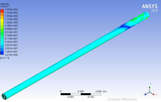
Based on setup made above simulation of the required system were run and result in terms of fluid velocity has been shown below.

According to the result flow of fluid inside the pipe will be turbulent as different velocities can be seen near inlet of the pipe along with the waves on entire length and especially on the top section of fluid domain.

It can be observed from the below mention figures that flow of fluid inside pipe is uniform and very smooth. This is due to the fact that wall roughness of the pipe is kept zero to make smooth pipe.

Experimental Results

Comparison

Moody chart mention below is used to find the frictional factor of the graphically and it is said to the ideal values of frictional factor as it does not consider the actual working conditions. 

For the initial velocity of 47.1 m/sec the experimental value of fractional factor is 0.0216 but for the calculated Reynold Number of 1*10^5 the graphical value is said to be 0.018 which quite less than the experimental value. 

The reason for high value of frictional factor in experiment is that pipe was considered smooth but it was not. Wall roughness of pipe add more value to frictional factor.

Discussion

The prediction made by the computational fluid dynamics for the behavior of the fluid flow is verified by the experimental data. 

Numerical analysis predicted that fluid flow will be turbulent in the pipe and according to the experimental results the calculated Reynold number for all initial velocities is above 4000 range which is for turbulent flow. 

This turbulent flow in smooth pipe is due to the high initial velocity as compared to the density of air.

According to the moody chart the frictional factor and Reynold number are connected to each other. So in order to find the relationship between these two a graph was generated which have friction factor on y axis and Reynold number on x axis. 

According to the trend shown in graph frictional factor and Reynold number are directly proportional to each other. Increase in value of Reynold number will increase the value of frictional factor and decrease in value of Reynold number will decrease the value of frictional factor

In order to find the relationship between mass flow rate and pressure drop a graph was generated which have pressure drop on y axis and mass flow rate on x axis. 

According to the trend shown in graph mass flow rate and pressure drop are directly proportional to each other. Increase in value of mass flow rate will increase the value of pressure drop and decrease in value of mass flow rate will decrease the value of pressure drop.